
In clinical neuroscience that deals with multiple psychiatric disorders, the influence of covariates on fMRI statistics can be pretty severe. It is common for things like a 20 year difference in mean age between groups to exist, which is known to create sizable group differences that have nothing to do with the diagnostic in question.
However, the common toolkits available for standard phrenology (or statistical parametric mapping) either don’t handle multiple covariates well (AFNI), or aren’t easy to apply to 100s of datasets (SPM, FSL). To remedy this, I created a set of command line tools to generate the prerequisites for FSL’s randomize and perform post-hoc cluster-size thresholding.
Overview
The process requires a database.csv with your input stat maps, group identifiers, and relevant covariates.
| filename | group | age | sex |
|---|---|---|---|
| corr_1.nii.gz | CTRL | 20 | 1 |
| corr_2.nii.gz | SCZ | 54 | 2 |
| corr_3.nii.gz | CTRL | 23 | 2 |
| corr_4.nii.gz | SCZ | 34 | 1 |
| corr_5.nii.gz | SCZ | 44 | 1 |
| corr_6.nii.gz | CTRL | 28 | 2 |
epi-design-maker: takes yourdatabase.csvand generates the inputs for the FSL GLM GUI.epi-randomize: takes a file with all of your inputs and the FSL design files generated by the FSL GLM GUI to run randomize. This outputs TFCE and uncorrected p-values with the associated t-stats for each contrast as a single concatenated file.epi-cluster: takes the concatenated p/t value file from the previous step, along with a voxel-extent and p-value threshold to produce cluster masks and reports for each contrast.
This process is almost entirely scrip-table, and I find it substantially easier to apply than the standard FSL method, which assumes you have used FSL for your pre-processing. In particular, this greatly speeds up the FSL GUI when you are trying to analyze many subjects, and allows you to easily try multiple threshold procedures post randomize, which can take over a day to run on a single machine.
Walkthrough
In this example, we’re interested in comparing seed-based connectivity of some brain region during rest across 4 diagnostic groups. We have 300 subjects total, which we preprocessed using a custom script (in this case, generated using epitome) and are now all in MNI space. I put them in the data/ folder with names like 201543_func-mni.nii.gz, where 201543 is the subject ID. I also have a group-wide brain mask called anat_mni_mask.nii.gz.
After producing a single MNI-space seed mask, producing the seed-based correlations is trivial with epi-seed-corr:
for run in $(ls data/*func-mni*); do
# get subject name
subj=$(basename ${run})
subj=$(echo ${subj} | cut -d '_' -f 1)
# run seeds
if [ ! -f seeds/${subj}_corr.nii.gz ]; then
epi-seed-corr ${run} seed_mask.nii.gz anat_mni_mask.nii.gz seeds/${subj}_corr.nii.gz
fi
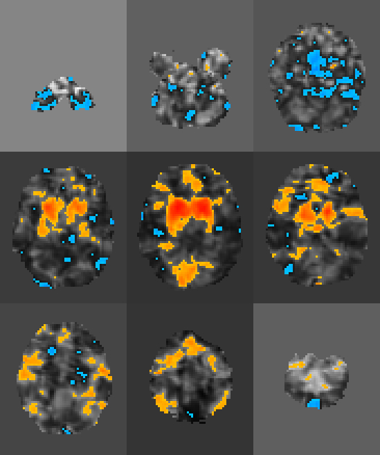
doneThis will produce a series of stat maps in seeds/. Here’s one as an example:
The next step is to create a .csv. that contains all of the information of interest. Because I had a lot of subjects, and I already had a .csv. containing all of the clinical variables and subject IDs, I could do the following to start my database.csv:
datapath='/srv/data/seeds'
output='database.echo'
csv 'subject,filename' > ${output}

for filename in $(ls ${datapath}); do
    subj=$(echo $(basename ${filename}) | cut -d '_' -f 1)
    echo ${subj},${filename} >> ${output}
done
Followed by a quick merge with the clinical variables in R:
database <- read.csv('database.csv')
data.to.add <- read.csv('full_spreadsheet.csv')
x <- merge(database, data.to.add, by='subject', all.x=TRUE)
write.csv(x, 'database-merged.csv')
Which produces a table that might look something like this (but with 300 rows):
| subject | filename | group | age | sex | medication |
|---|---|---|---|---|---|
| 201543 | /srv/data/seeds/201543_corr.nii.gz | CTRL | 20 | 1 | grokapine |
| 101565 | /srv/data/seeds/101565_corr.nii.gz | SCZ | 54 | 2 | slockapine |
| 200232 | /srv/data/seeds/200232_corr.nii.gz | CTRL | 23 | 2 | grokapine |
| 104323 | /srv/data/seeds/104323_corr.nii.gz | PSY | 34 | 1 | graphicle |
| 105346 | /srv/data/seeds/105346_corr.nii.gz | PSY | 44 | 1 | slopicle |
| 202223 | /srv/data/seeds/202223_corr.nii.gz | BPD | 28 | 2 | slockapine |
The next step is to create two files to use with FSL. The first will be a list of input files (the filename column) and the second will be the full design matrix that FSL needs to run randomize. This full design matrix will not only include the columns for each group, but also the dummy variables for each covariate of no-interest. In this analysis, we want to center the age covariate for each group separately, because the mean age is going to be different for each diagnosis. This is done by specifying the covariate with an @ tacked onto the end.
epi-design-maker database-merged.csv age@ sexthis is the only non-scriptable part of the analysis
This outputs fsl_subjects.txt and fsl_design.txt, which can be pasted directly into the FSL GLM GUI, our next stop. In FSL, after pasting these large files into the GUI (take advantage of the ‘paste’ button to save yourself a lot of headache), you can go about defining the contrasts you want to run. Finally, save the design, which should output a .con, .grp, and .mat file, among others. Now to run randomize with a bunch of permutations, do something like this:
epi-randomize \
    --prefix=rand \
    --n=5000 \
    --design=fsl_glm.mat \
    --contrasts=fsl_glm.con \
    --group=fsl_glm.grp \
    --cleanup \
    fsl_subjects.txt
For a 300 subject experiment with a good number of contrasts (say, 14), this procedure can take a long time, upwards of a day on a single machine. However it will conveniently output all of the contrasts stats in a single concatenated file for exploration later.
This single file can be thresholded anyways you want (the tstat pstat files are alternating, in pairs). However, one decent method would be using cluster-size thresholding based on a Monte Carlo simulation of the expected null stat sizes.
In this case, we first estimate the smoothness of each input functional file (the ones we used to generate the correlation maps). This can be done pretty easily with AFNI’s 3dFWHMx:
output='fwhm.csv'

echo '#x y z' > ${output}
for run in $(ls data/*func-mni*); do
    xyz=$(3dFWHMx -mask anat_MNI_mask.nii.gz -demean -input ${run})
    echo ${xyz} >> ${output}
done
Now we can compute the mean smoothness in the x, y, and z dimensions across all of our subjects:
import numpy as np

x = np.genfromtxt('fwhm.csv', skip_header=1)
x = np.mean(x, axis=0)
np.savetxt('fwhm-means.csv', x)
And finally run the Monte Carlo cluster simulation using AFNI’s 3dClustSim:
x=$(cat fwhm-means.csv | head -1 | xargs)
y=$(cat fwhm-means.csv | head -2 | tail -1 | xargs)
z=$(cat fwhm-means.csv | tail -1 | xargs)

3dClustSim \
    -mask anat_mni_mask.nii.gz \
    -fwhmxyz ${x} ${y} ${z} \
    -iter 10000 \
    -nodec \
    -prefix clust_sizes.1D
Which will output a file that looks something like this:
# Grid: 61x73x61 3.00x3.00x3.00 mm^3 (70766 voxels in mask)
#
# CLUSTER SIZE THRESHOLD(pthr,alpha) in Voxels
# -NN 1  | alpha = Prob(Cluster >= given size)
#  pthr  | .10000 .05000 .02000 .01000
# ------ | ------ ------ ------ ------
 0.020000     222    259    306    335
 0.010000     132    154    182    200
 0.005000      85    101    122    136
 0.002000      51     62     75     87
 0.001000      36     44     54     63
 0.000500      25     31     40     47
 0.000200      15     20     26     32
 0.000100      10     14     19     24
This is a pretty useful table. The left column has a list of uncorrected p thresholds, and the top has a list of alpha levels. The values in the table are the number of connected voxels at a given p value required to satisfy some alpha level. We’re going to assume you’re hoping to publish with an alpha of 0.05. Depending on our hypothesis, we might expect our significant regions to be small (say some subcortical region), or large (the dorsolateral prefrontal cortex). If they are large, we can relax our p threshold (say to 0.02) and look for clusters with > 259 voxels. If they are small, we can set our p threshold to something like 0.0005 and look for clusters with > 31 voxels. This stage might take a few different tries to see how the data looks under different conditions, which is why the epi-cluster tool is separate from the long-running epi-randomize.
To produce thresholded stat maps with a given cluster threshold, try the following:
epi-cluster --n=101 --p=0.005 --pflip randomize_rand_raw.nii.gzWhich will produce a set of stat_cluster_${contrast_number}.nii.gz files from your randomize input. If a cluster map is empty, they will be very small .nii.gz files when compared with their peers (since zeros are not stored in .gz files). Here is an example output: a thresholded t-map of the 10th contrast (group SCZ - BPD):
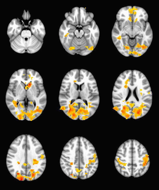
This procedure can be used to run a very large number of subjects through FSL’s randomize with very little pain in the data-preparation stage, and has the added benefit of being compatible with any pre-processing procedure or statistical map. Since randomize is very flexible about the kinds of statistics it can work with, you can use these tools in combination with your favorite analysis techniques and tool chains to run MRI analysis on sizable populations.